Checking Your Cooper and Jacob Match

Groundwater hydrologists use the Cooper and Jacob (1946) solution to determine the aquifer properties of a nonleaky confined aquifer using drawdowns measured during a constant-rate pumping test. The approximate method of Cooper and Jacob derives from the Theis (1935) type-curve method when the variable u in the Theis well function, w(u), is sufficiently small (i.e., time is large or radius is small).

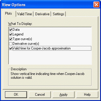
AQTESOLV has built-in tools to check the validity of analyses performed with the Cooper and Jacob method and to assist you with visual curve matching. First, you can superimpose on your plot the time when u is less than a critical value. Choose View>Options>Plots tab and check the option for Valid time for Cooper-Jacob approximation (Figure 1).

Figure 1. Check option to display valid time for Cooper and Jacob solution.

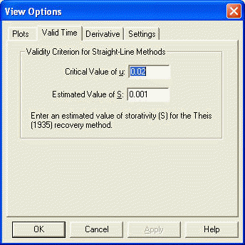
Click the Valid Time tab to set the critical value of u (Figure 2). A critical value between 0.01 and 0.05 is typical.

Figure 2. Set critical value of u used to check validity of Cooper and Jacob approximation.

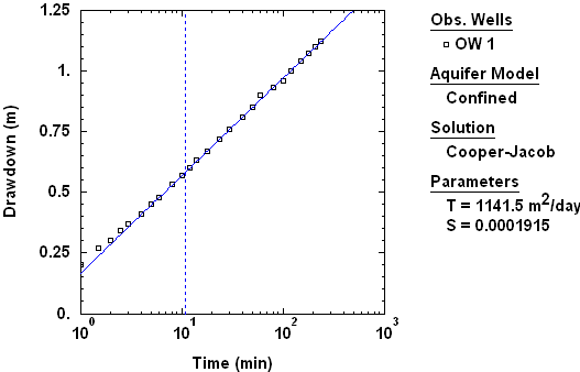
When you activate the valid time option, a dashed vertical line appears on your time-drawdown or composite plot to indicate the time when the Cooper and Jacob approximation meets the critical value of u (Figure 3). The position of the vertical line is a function of T (transmissivity) and S (storage coefficient) as well as radial distance between the pumping and observation wells..

Figure 3. Cooper and Jacob method (blue line) matched to time-drawdown data from constant-rate pumping test (data from Todd 1980). Dashed vertical line indicates time when Cooper and Jacob approximation becomes valid.

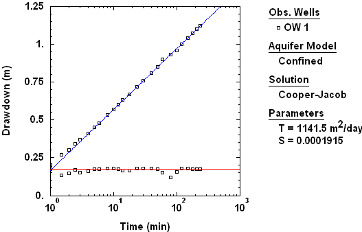
The second way that you may evaluate the proper application of the Cooper and Jacob method using AQTESOLV is through derivative analysis. After superimposing the derivative on your semilog plot of drawdown versus time, match the Cooper and Jacob straight line to drawdowns corresponding to the derivative plateau, i.e., during the period of infinite-acting radial flow (Figure 4).

Figure 4. Cooper and Jacob method (blue line) matched to drawdown data during period of infinite-acting radial flow when derivative reaches plateau (red line).

Use these two techniques to obtain more reliable results when using the Cooper and Jacob method. Get AQTESOLV and start applying these powerful tools in your next pumping test interpretation!

Visit the AQTESOLV Knowledge Base to find more tips on the using the software. The AQTESOLV documentation also includes a number of examples illustrating the use of the Cooper and Jacob straight-line method.

We invite you to follow HydroSOLVE on LinkedIn and Google+!

IARF and the Cooper and Jacob Method

Groundwater hydrologists routinely use the pumping test interpretation method of Cooper and Jacob (1946), a straight-line approximation of the Theis (1935) type-curve solution, to estimate the hydraulic properties of nonleaky confined aquifers from drawdown data measured during the period of infinite-acting radial flow (IARF) when drawdown changes linearly with the logarithm of time. One expects to find IARF after the dissipation of early-time phenomena (e.g., wellbore storage) and prior to the advent of late-time effects such as aquifer boundaries.

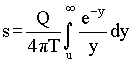
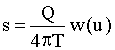
Consider the well-known Theis solution for a constant-rate pumping test in a nonleaky confined aquifer of infinite extent:

..... (1)

..... (2)

..... (3)

..... (4)

where s is drawdown [L], Q is pumping rate [L³/T], T is transmissivity [L²/T], t is time [T], r is radial distance [L] and S is storage coefficient [-].

The Cooper and Jacob method approximates the Theis well function, w(u), by truncating the infinite series in (4) after the first two terms:

..... (5)

The approximation in (5) assumes that u is small, i.e., t is large and r is small. It is precisely when (5) is valid that infinite-acting radial flow is identified from drawdown data.

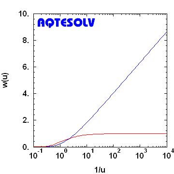
How small should u be for (5) to be valid? The threshold for IARF (i.e., when Cooper and Jacob becomes valid) is often given as u ≤ 0.05 (Driscoll 1986) or u ≤ 0.01 (Kruseman and de Ridder 1994); however, we can see for ourselves when (5) is valid by plotting w(u) versus 1/u (dimensionless drawdown versus dimensionless time) on semilog axes and looking for a constant logarithmic derivative plateau (Figure 1).

Figure 1. Theis (1935) solution (blue curve) plotted as w(u) versus 1/u on semilog axes. Logarithmic derivative shown by red curve.

It is evident from Figure 1 that the slope of the drawdown and the value of the derivative are each essentially constant when 1/u ≥ 50. Hence, when u ≤ 0.02, the Cooper and Jacob approximation of the Theis well function is safe to use. Figure 1 demonstrates just how useful derivative analysis can be for the detection of the IARF regime.

Visit Aquifer Testing 101 to learn more about pumping test interpretation with more examples of infinite-acting radial flow.

Follow HydroSOLVE on LinkedIn and Google+!