Checking Your Cooper and Jacob Match

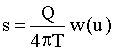
Groundwater hydrologists use the Cooper and Jacob (1946) solution to determine the aquifer properties of a nonleaky confined aquifer using drawdowns measured during a constant-rate pumping test. The approximate method of Cooper and Jacob derives from the Theis (1935) type-curve method when the variable u in the Theis well function, w(u), is sufficiently small (i.e., time is large or radius is small).

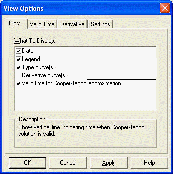
AQTESOLV has built-in tools to check the validity of analyses performed with the Cooper and Jacob method and to assist you with visual curve matching. First, you can superimpose on your plot the time when u is less than a critical value. Choose View>Options>Plots tab and check the option for Valid time for Cooper-Jacob approximation (Figure 1).

Figure 1. Check option to display valid time for Cooper and Jacob solution.

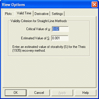
Click the Valid Time tab to set the critical value of u (Figure 2). A critical value between 0.01 and 0.05 is typical.

Figure 2. Set critical value of u used to check validity of Cooper and Jacob approximation.

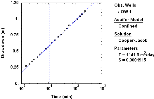
When you activate the valid time option, a dashed vertical line appears on your time-drawdown or composite plot to indicate the time when the Cooper and Jacob approximation meets the critical value of u (Figure 3). The position of the vertical line is a function of T (transmissivity) and S (storage coefficient) as well as radial distance between the pumping and observation wells..

Figure 3. Cooper and Jacob method (blue line) matched to time-drawdown data from constant-rate pumping test (data from Todd 1980). Dashed vertical line indicates time when Cooper and Jacob approximation becomes valid.

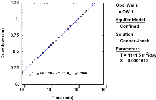
The second way that you may evaluate the proper application of the Cooper and Jacob method using AQTESOLV is through derivative analysis. After superimposing the derivative on your semilog plot of drawdown versus time, match the Cooper and Jacob straight line to drawdowns corresponding to the derivative plateau, i.e., during the period of infinite-acting radial flow (Figure 4).

Figure 4. Cooper and Jacob method (blue line) matched to drawdown data during period of infinite-acting radial flow when derivative reaches plateau (red line).

Use these two techniques to obtain more reliable results when using the Cooper and Jacob method. Get AQTESOLV and start applying these powerful tools in your next pumping test interpretation!

Visit the AQTESOLV Knowledge Base to find more tips on the using the software. The AQTESOLV documentation also includes a number of examples illustrating the use of the Cooper and Jacob straight-line method.

We invite you to follow HydroSOLVE on LinkedIn and Google+!

IARF and the Cooper and Jacob Method

Groundwater hydrologists routinely use the pumping test interpretation method of Cooper and Jacob (1946), a straight-line approximation of the Theis (1935) type-curve solution, to estimate the hydraulic properties of nonleaky confined aquifers from drawdown data measured during the period of infinite-acting radial flow (IARF) when drawdown changes linearly with the logarithm of time. One expects to find IARF after the dissipation of early-time phenomena (e.g., wellbore storage) and prior to the advent of late-time effects such as aquifer boundaries.

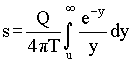
Consider the well-known Theis solution for a constant-rate pumping test in a nonleaky confined aquifer of infinite extent:

..... (1)

..... (2)

..... (3)

..... (4)

where s is drawdown [L], Q is pumping rate [L³/T], T is transmissivity [L²/T], t is time [T], r is radial distance [L] and S is storage coefficient [-].

The Cooper and Jacob method approximates the Theis well function, w(u), by truncating the infinite series in (4) after the first two terms:

..... (5)

The approximation in (5) assumes that u is small, i.e., t is large and r is small. It is precisely when (5) is valid that infinite-acting radial flow is identified from drawdown data.

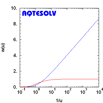
How small should u be for (5) to be valid? The threshold for IARF (i.e., when Cooper and Jacob becomes valid) is often given as u ≤ 0.05 (Driscoll 1986) or u ≤ 0.01 (Kruseman and de Ridder 1994); however, we can see for ourselves when (5) is valid by plotting w(u) versus 1/u (dimensionless drawdown versus dimensionless time) on semilog axes and looking for a constant logarithmic derivative plateau (Figure 1).

Figure 1. Theis (1935) solution (blue curve) plotted as w(u) versus 1/u on semilog axes. Logarithmic derivative shown by red curve.

It is evident from Figure 1 that the slope of the drawdown and the value of the derivative are each essentially constant when 1/u ≥ 50. Hence, when u ≤ 0.02, the Cooper and Jacob approximation of the Theis well function is safe to use. Figure 1 demonstrates just how useful derivative analysis can be for the detection of the IARF regime.

Visit Aquifer Testing 101 to learn more about pumping test interpretation with more examples of infinite-acting radial flow.

Follow HydroSOLVE on LinkedIn and Google+!

Infinite-Acting Radial Flow Regime

At the outset of interpreting a pumping test, an important feature to detect in the response data is infinite-acting radial flow. During infinite-acting radial flow, steady pumping in a nonleaky confined aquifer of infinite extent produces late-time drawdown that changes with the logarithm of time since pumping began. Infinite-acting behavior occurs after wellbore storage effects have dissipated and before the influence of aquifer boundaries. One may observe this flow regime by plotting the familiar Theis (1935) solution on semilog axes (Figure 1); at late time, a graph of dimensionless drawdown, w(u), versus dimensionless time, 1/u, plots as a straight line and the logarithmic derivative is constant.

 

Figure 1. Infinite-acting radial flow in a nonleaky confined aquifer illustrated with Theis (1935) solution (dimensionless drawdown and dimensionless derivative shown by blue and red curves, respectively).

This late-time behavior of the Theis model is well known to groundwater hydrologists. The period of infinite-acting radial flow is the basis for the tried-and-true Cooper and Jacob (1946) method which one may use to find the transmissivity and storage coefficient of a nonleaky confined aquifer by matching a straight line to late-time drawdown data from a constant-rate pumping test plotted on semilog axes.

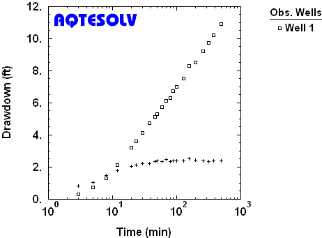
A derivative plot is very useful for detecting the infinite-acting radial flow regime under steady pumping conditions. One starts by looking for a derivative plateau (constant derivative) to tentatively identify infinite-acting radial flow. For example, the response data from a constant-rate pumping test shown in Figure 2 suggest that infinite-acting radial flow conditions are present after approximately 30 minutes of pumping once the derivative stabilizes.

Figure 2. Derivative plot of drawdown (squares) and derivative (crosses) measured in an observation well during constant-rate pumping test in a nonleaky confined aquifer (Walton 1962).

Note that the derivative plateau in Figure 2 exhibits some noise; derivative fluctuation at the plateau is common in the application of derivative analysis, but the presence of a near-constant derivative in this example is clear and corresponds to the emergence of a well-defined straight line in the drawdown data.

The foregoing results suggest that the derivative plot is an indispensable tool for aquifer test interpretation; however, the mere existence of a derivative plateau does not immediately confirm infinite-acting radial flow conditions. For example, an aquifer limited by a no-flow boundary can produce a constant derivative that is not diagnostic of the infinite-acting radial flow regime. In such a situation, geologic mapping of lithologic contacts, faults and other low-permeability features would be invaluable in making a correct interpretation.

Visit Aquifer Testing 101 for a catalog of derivative plot signatures with more examples of infinite-acting radial flow in pumping tests.

Follow HydroSOLVE on LinkedIn!

Catalog of Derivative Plots

Derivative analysis is a powerful diagnostic technique for the interpretation of data from pumping tests. Use of the derivative in pumping test analysis can highlight many flow regime features that otherwise may be hard to discover when inspecting drawdown data alone.

A catalog of derivative plots, showing the theoretical drawdown and derivative signatures on log-log axes for different flow regimes, is a useful reference to the practicing hydrogeologist when performing derivative analysis. For example, Figure 1 shows the drawdown and derivative response for a finite-diameter pumping well with wellbore storage in an infinite nonleaky confined aquifer.

Figure 1. Wellbore storage flow regime, infinite nonleaky confined aquifer.

One observes the wellbore storage flow regime at early time when the drawdown and derivative curves both exhibit unit (1:1) slopes (Figure 1). Radial flow in an infinite-acting aquifer shows up as a plateau on the derivative response.

An extensive catalog of derivative plots is available at the Aquifer Testing 101 section of the AQTESOLV web site to help you with derivative analysis. Use the catalog to become familiar with the derivative plot signatures for various well/aquifer geometries corresponding to different flow regimes.

Importance of Smoothing Derivative Data

Derivative analysis is a powerful diagnostic tool that enhances the interpretation of pumping test data. Hydrogeologists use the technique to identify flow regimes, discern boundary conditions and refine the selection of aquifer models.

Derivatives are not measured directly in the field; rather, they are computed by numerical differentiation from drawdowns collected during a pumping test. Straightforward calculation of the derivative from neighboring drawdown measurements typically leads to noisy derivative data. Therefore, smoothing routines are employed to obtain a cleaner derivative signal (Bourdet et al. 1989; Spane and Wurstner 1993).

To appreciate the importance of derivative smoothing, consider field data measured in a deep piezometer during a constant-rate pumping test performed in an unconfined aquifer (Kruseman and de Ridder 1994). Figure 1 is a derivative plot for the piezometer showing drawdown (squares) and derivatives (crosses) computed without smoothing (nearest neighbor method). Without smoothing, the derivative data provide little useful information for the interpretation of this test.

Figure 1. Derivative plot showing derivatives computed without smoothing.

Application of the Bourdet method to smooth the derivatives leads to a derivative plot with useful information (Figure 2). The trough in the derivative curve shown in Figure 2 is typical for an unconfined aquifer with delayed yield. The derivative signature suggests the possibility of using a mathematical model by Neuman (1974) to interpret the data.

Figure 2. Derivative plot showing derivatives computed with Bourdet smoothing.

AQTESOLV features three smoothing methods for computing derivatives including the Bourdet and Spane methods.

More information on derivative analysis is available at Aquifer Testing 101.