When using AQTESOLV to perform visual curve matching on a data set with multiple observation wells, it's often useful to turn off the display of one or more wells and focus your attention on the remaining wells.
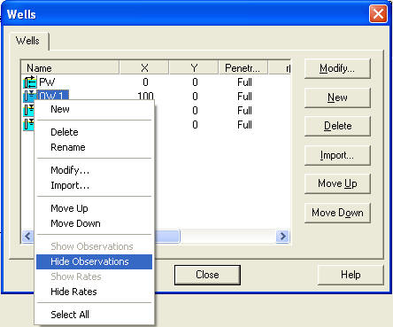
To hide observation data for particular wells, choose Edit>Wells and select the wells in the list that you'd like to hide. Right click over the selection and choose Hide Observations.
To turn on the display of hidden observations wells, select the wells to display, right click over the selection and choose Show Observations.
Find more tips on the AQTESOLV website!
Follow AQTESOLV on LinkedIn and Google+!
Showing posts with label tips. Show all posts
Tuesday, February 25, 2014
Wednesday, February 5, 2014
Checking Your Cooper and Jacob Match
Groundwater hydrologists use the Cooper and Jacob (1946) solution to determine the aquifer properties of a nonleaky confined aquifer using drawdowns measured during a constant-rate pumping test. The approximate method of Cooper and Jacob derives from the Theis (1935) type-curve method when the variable u in the Theis well function, w(u), is sufficiently small (i.e., time is large or radius is small).
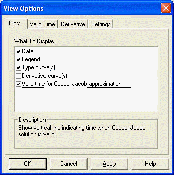
AQTESOLV has built-in tools to check the validity of analyses performed with the Cooper and Jacob method and to assist you with visual curve matching. First, you can superimpose on your plot the time when u is less than a critical value. Choose View>Options>Plots tab and check the option for Valid time for Cooper-Jacob approximation (Figure 1).
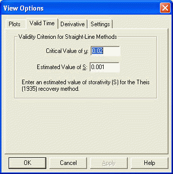
Click the Valid Time tab to set the critical value of u (Figure 2). A critical value between 0.01 and 0.05 is typical.
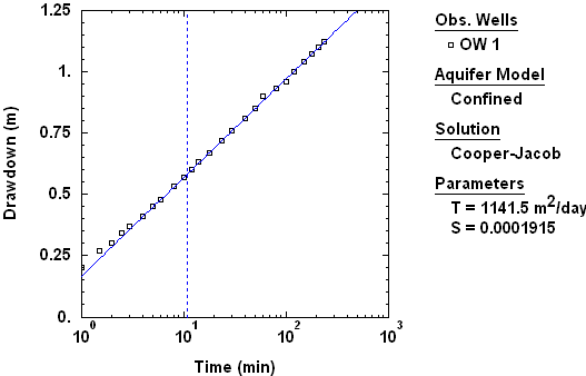
When you activate the valid time option, a dashed vertical line appears on your time-drawdown or composite plot to indicate the time when the Cooper and Jacob approximation meets the critical value of u (Figure 3). The position of the vertical line is a function of T (transmissivity) and S (storage coefficient) as well as radial distance between the pumping and observation wells..
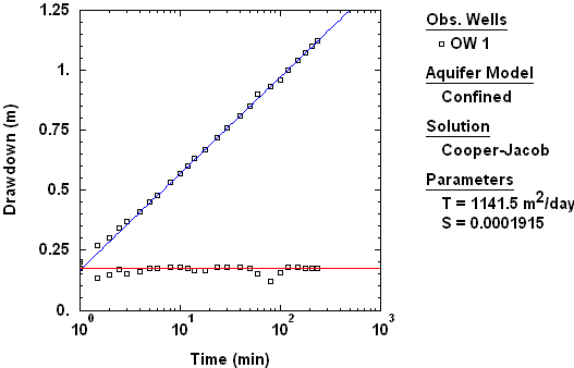
derivative analysis. After superimposing the derivative on your semilog plot of drawdown versus time, match the Cooper and Jacob straight line to drawdowns corresponding to the derivative plateau, i.e., during the period of infinite-acting radial flow (Figure 4).
Use these two techniques to obtain more reliable results when using the Cooper and Jacob method. Get AQTESOLV and start applying these powerful tools in your next pumping test interpretation!
Visit the AQTESOLV Knowledge Base to find more tips on the using the software. The AQTESOLV documentation also includes a number of examples illustrating the use of the Cooper and Jacob straight-line method.
We invite you to follow HydroSOLVE on LinkedIn and Google+!
AQTESOLV has built-in tools to check the validity of analyses performed with the Cooper and Jacob method and to assist you with visual curve matching. First, you can superimpose on your plot the time when u is less than a critical value. Choose View>Options>Plots tab and check the option for Valid time for Cooper-Jacob approximation (Figure 1).
| Figure 1. Check option to display valid time for Cooper and Jacob solution. |
| Figure 2. Set critical value of u used to check validity of Cooper and Jacob approximation. |
derivative analysis. After superimposing the derivative on your semilog plot of drawdown versus time, match the Cooper and Jacob straight line to drawdowns corresponding to the derivative plateau, i.e., during the period of infinite-acting radial flow (Figure 4).
| Figure 4. Cooper and Jacob method (blue line) matched to drawdown data during period of infinite-acting radial flow when derivative reaches plateau (red line). |
Visit the AQTESOLV Knowledge Base to find more tips on the using the software. The AQTESOLV documentation also includes a number of examples illustrating the use of the Cooper and Jacob straight-line method.
We invite you to follow HydroSOLVE on LinkedIn and Google+!
Tuesday, December 10, 2013
Curve Matching With Multiple Observation Wells
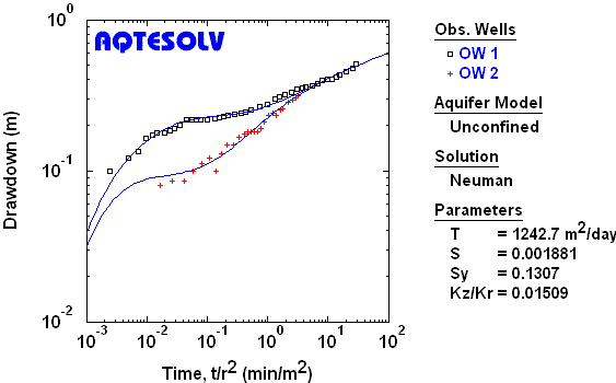
When you analyze a pumping test with more than one observation well, AQTESOLV matches one set of aquifer properties to the drawdown data from all of the wells in your data set.
In the figure shown above, the curve-fitting analysis determines the properties of an unconfined aquifer with delayed yield from the two observation wells displayed on the graph.
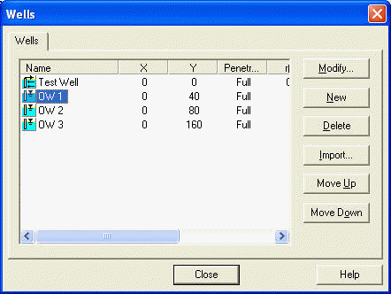
Of course, if your data set has multiple observation wells, you may match wells individually or in groups with AQTESOLV as well. To perform visual curve matching on selected wells, choose Wells from the Edit menu to see all of the wells in your data set. Right click over a well in the list and choose Hide Observations to turn off the display of the well; to turn on the display a previously hidden well, choose Show Observations when you right click over a well.
To select more than one well at a time, hold down the Ctrl key when clicking on wells in the list shown above.
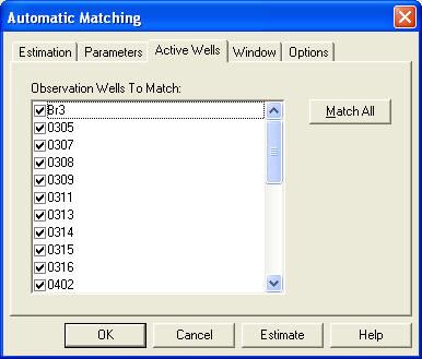
AQTESOLV allows you to select which wells to use for automatic curve matching, too. Choose Automatic from the Match menu and click the Active Wells tab. Remove the check next to any well that you wish to ignore during automatic matching.
Selections in the Active Wells list shown above only affect the wells used for automatic matching, not the display of well data.
Visit the Support Center and the Knowledge Base at the AQTESOLV website for additional tips and examples.
| One set of aquifer properties matched to two observation wells from a constant-rate pumping test in an unconfined aquifer with delayed yield. |
Of course, if your data set has multiple observation wells, you may match wells individually or in groups with AQTESOLV as well. To perform visual curve matching on selected wells, choose Wells from the Edit menu to see all of the wells in your data set. Right click over a well in the list and choose Hide Observations to turn off the display of the well; to turn on the display a previously hidden well, choose Show Observations when you right click over a well.
| Choose Edit>Wells to add, modify or delete wells from an AQTESOLV data set. |
AQTESOLV allows you to select which wells to use for automatic curve matching, too. Choose Automatic from the Match menu and click the Active Wells tab. Remove the check next to any well that you wish to ignore during automatic matching.
| Choose Match>Automatic>Active Wells to select wells to match with automatic curve matching. |
Visit the Support Center and the Knowledge Base at the AQTESOLV website for additional tips and examples.
Tuesday, November 26, 2013
Entering Pumping Rates Into AQTESOLV
Entering pumping rates from an aquifer test into AQTESOLV requires little effort. The first thing to remember is that all pumping rates are entered as a sequence of constant-rate steps. For each step, enter the time when the step begins (as elapsed time since the start of the test) with the corresponding pumping rate. For your convenience, AQTESOLV provides options to type the rates into a spreadsheet, import them from a file or copy/paste them from another spreadsheet.
Constant-Rate Test
Constant-Rate Test With Recovery
Variable-Rate Test
Constant-Rate Test
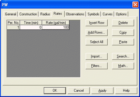
For a constant-rate pumping test, you only need to enter one rate into AQTESOLV. For example, if the pumping rate during a constant-rate test is 100 gpm (gallons-per-minute), enter the rate as shown below.
| Pumping rate entry for a constant-rate test. |
Note that there's no need to duplicate the rate in the spreadsheet after the first entry. AQTESOLV assumes that the rate doesn't change until you add a new one. Duplicating rates in successive rows of the spreadsheet only serves to slow down calculations.
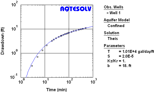
The following figure shows an interpretation of drawdown data from a constant-rate pumping test with the Theis (1935) type-curve method.
| Analysis of drawdown data from constant-rate pumping test. |
Constant-Rate Test With Recovery
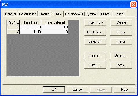
Now consider a constant-rate pumping test with recovery. For this case, enter the constant-rate portion of the test as above and add a row to the rates spreadsheet to indicate the start of recovery. For example, if pumping at 100 gpm ceases after 24 hours (1440 minutes), enter the constant rate and recovery periods as follows.
| Pumping rate entry for a constant-rate test with recovery. |
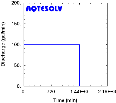
The next graph shows the rate history for the example above. The rate during the pumping test is a constant 100 gpm. After one day (1440 minutes), the test ends and the rate is zero during recovery.
| Rate history for constant-rate test with recovery. |
As before, do not duplicate pumping rates in successive rows of the rates spreadsheet. Between 0 and 1440 minutes, AQTESOLV recognizes that the constant rate is 100 gpm. AQTESOLV knows from the data entered that the rate after 1440 minutes is zero during recovery.
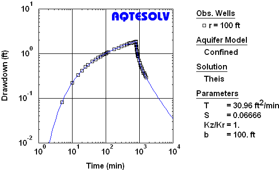
The plot below illustrates the analysis of drawdown and recovery data from a constant-rate pumping test with recovery.
| Analysis of constant-rate pumping test with recovery. |
Variable-Rate Test
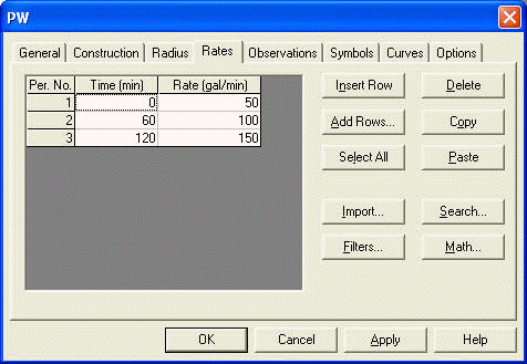
Entering pumping rates for a variable-rate test is likewise straightforward. Enter a new rate into AQTESOLV when the rate changes. For example, consider a step-drawdown test consisting of three one-hour steps of 50, 100 and 150 gpm. As before, the first step starts at an elapsed time of zero. The second and third steps begin at 60 and 120 minutes, respectively.
| Pumping rate entry for step-drawdown test. |
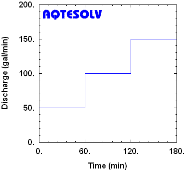
The rate history for this step-drawdown test example is illustrated in the graph below.
| Rate history for step-drawdown test. |
Enter only one row per step in the rates spreadsheet to indicate when the step begins. During each step, the pumping rate is assumed to remain constant.
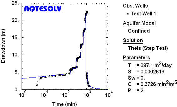
Interpretation of a step-drawdown test with recovery is shown in the following figure.
| Interpretation of drawdown and recovery data from a step-drawdown test. |
Visit the Knowledge Base at the AQTESOLV website for more helpful tips on using the software!
Tuesday, November 19, 2013
AQTESOLV Examples and Tutorials
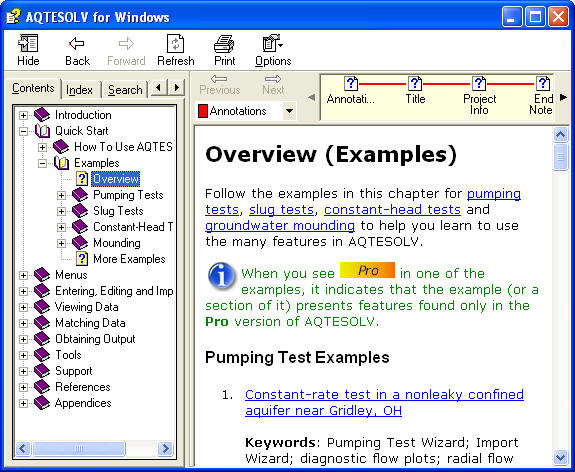
The Help file installed with AQTESOLV is chock-full of examples with step-by-step instructions for using the software.
To access the Help system, choose Contents and Index from the Help menu in the AQTESOLV application. Go to the Quick Start chapter in the Contents tab to explore the many detailed tutorials for analyzing pumping tests, slug tests and constant-head tests.
To download a PDF version of the AQTESOLV manual, please visit the Support Center at the AQTESOLV website.
| Accessing Examples in the AQTESOLV Help System |
To download a PDF version of the AQTESOLV manual, please visit the Support Center at the AQTESOLV website.
Wednesday, November 13, 2013
Intermittent Pumping
One of the many applications for the variable pumping rate option in AQTESOLV is to simulate drawdown resulting from intermittent pumping in one or more pumping wells. Use this feature for pumping test interpretation or drawdown modeling.
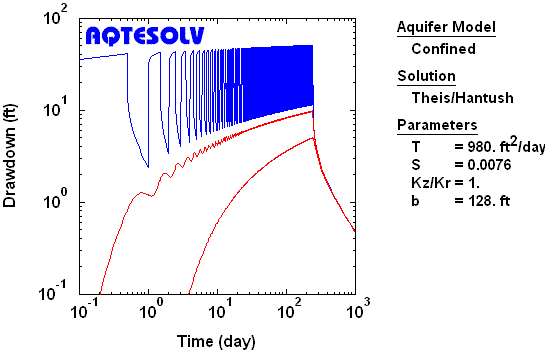
In the following figure, AQTESOLV predicts drawdown due to an irrigation well extracting water from a nonleaky confined aquifer with daily on/off cycles extending over a growing season of 245 days. During each pumping cycle, the well withdraws groundwater at 220 gallons-per-minute (gpm) for 12 hours followed by 12 hours of recovery. At the end of the growing season, all pumping stops and sustained recovery begins. Drawdown in the pumping well (blue line) clearly shows the cycles of intermittent pumping; whereas the two observation wells (red lines) located 500 and 2000 ft from the extraction well demonstrate how the cyclic drawdown response dissipates with distance.
Entering a lot of pumping cycles by hand can be tedious, so AQTESOLV makes the task easy for you. One method is to prepare the cyclic rate history in Excel and copy/paste the rates from Excel into AQTESOLV. Alternatively, you may enter just one cycle into AQTESOLV and have the software repeat the cycle a specified number of times (find details in the AQTESOLV manual).
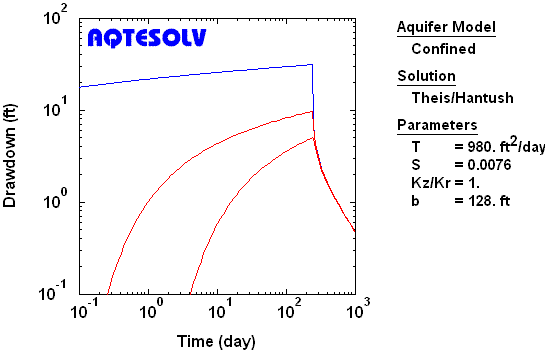
If your primary interest is the average drawdown at relatively distant observation wells over long periods of intermittent pumping, it is often sufficient to assume a constant average pumping rate. The following figure shows the predicted drawdown for a well extracting at 110 gpm over the same 245-day growing season as the previous intermittent pumping scenario.
The two preceding examples applied the Theis (1935) nonequilibrium solution to predict drawdown under intermittent pumping conditions in a nonleaky confined aquifer of infinite extent; however, you may use virtually any of the pumping test solutions in AQTESOLV to forecast drawdown for constant- or variable-rate pumping in nonleaky confined, leaky confined, unconfined or fractured aquifers. Plus, AQTESOLV allows you to add no-flow or constant-head boundaries to model surface water boundaries and limited aquifers as required.
In the following figure, AQTESOLV predicts drawdown due to an irrigation well extracting water from a nonleaky confined aquifer with daily on/off cycles extending over a growing season of 245 days. During each pumping cycle, the well withdraws groundwater at 220 gallons-per-minute (gpm) for 12 hours followed by 12 hours of recovery. At the end of the growing season, all pumping stops and sustained recovery begins. Drawdown in the pumping well (blue line) clearly shows the cycles of intermittent pumping; whereas the two observation wells (red lines) located 500 and 2000 ft from the extraction well demonstrate how the cyclic drawdown response dissipates with distance.
| Drawdown due to intermittent (cyclic) pumping in a nonleaky confined aquifer. |
If your primary interest is the average drawdown at relatively distant observation wells over long periods of intermittent pumping, it is often sufficient to assume a constant average pumping rate. The following figure shows the predicted drawdown for a well extracting at 110 gpm over the same 245-day growing season as the previous intermittent pumping scenario.
| Drawdown assuming average pumping rate in a nonleaky confined aquifer. |
Wednesday, November 6, 2013
Distance-Drawdown Analysis
Distance-drawdown analysis is a useful technique for estimating aquifer properties when drawdown measurements are taken during a pumping test at several observation wells located at different radial distances from the control (pumped) well. To perform distance-drawdown analysis, one plots a single drawdown observation per well, each recorded at the same time since the start of pumping, on a graph of drawdown versus radial distance.
Most of us are familiar with estimating an aquifer's transmissivity and storativity from distance-drawdown data using the Cooper and Jacob (1946) method as shown in the following figure.
| Distance-drawdown analysis for an unconfined aquifer. |
Did you know that you may perform distance-drawdown analysis with pumping test methods in AQTESOLV other than Cooper and Jacob? For example, you may match distance-drawdown data with the Hantush and Jacob (1955) method for a leaky confined aquifer (see figure below).
To display a distance-drawdown graph in AQTESOLV, choose Distance-Drawdown from the View menu. The Distance-Drawdown option is active when you have more than one observation well in your data set. If your data set includes more than one pumping well, the Distance-Drawdown option is inactive as distance-drawdown analysis assumes radially symmetric flow around a single pumping well; however, you may use AQTESOLV to prepare contour plots of drawdown (plan and cross section) when multiple pumping wells are present.
To learn more about AQTESOLV, take the guided tour or download the demo!
| Distance-drawdown plot for a leaky confined aquifer. |
To learn more about AQTESOLV, take the guided tour or download the demo!
Wednesday, October 23, 2013
Plot Orientation in AQTESOLV
Many groundwater hydrologists prefer plotting drawdown data from a pumping test with the origin placed in the upper left corner of the graph. When formatted this way, a graph shows drawdown increasing downward.
To have AQTESOLV orient your drawdown plot in this manner, choose Format from the View menu and check Origin in Upper Left.
For additional AQTESOLV tips, visit the Knowledge Base and Examples at the AQTESOLV Support Center.
![]() |
| Analysis of drawdown and recovery from a pumping test in a confined aquifer. |
For additional AQTESOLV tips, visit the Knowledge Base and Examples at the AQTESOLV Support Center.
Tuesday, August 30, 2011
Enhancing Reliability of Slug Test Data Analysis
Data from an overdamped slug test in a well with a fully submerged screen (screen below water table) may exhibit a concave upward appearance on a plot of log normalized head vs. time. The curvature can make analysis by straight-line methods such as Bouwer and Rice (1976) somewhat ambiguous.
Butler (1998) suggests matching straight-line slug test solutions to data within recommended normalized head ranges to overcome ambiguity associated with slug test data curvature and thereby enhance the reliability of data analysis. AQTESOLV, advanced software for slug test analysis, includes the recommended normalized head ranges to assist you with visual curve matching.
Learn more about recommended normalized head ranges and slug testing in Aquifer Testing 101 at the AQTESOLV web site.
![]() |
| Analysis of slug test data using recommended normalized head range. |
Learn more about recommended normalized head ranges and slug testing in Aquifer Testing 101 at the AQTESOLV web site.
Thursday, July 14, 2011
Agarwal Recovery Method
In yesterday's post, I presented three different methods for analyzing recovery tests. Today, I will focus on the Agarwal recovery method which has been used by petroleum engineers for over 30 years. Agarwal (1980) devised a simple yet powerful data transformation for the interpretation of recovery tests. The transformation, known as Agarwal equivalent time, allows one to analyze recovery data with standard type curves developed for drawdown data.
The following figure illustrates the simplicity of the Agarwal method in the analysis of a recovery test. In this example, I matched the familiar Theis type curve, normally applied to drawdown data, to estimate aquifer properties from recovery test data (USBR 1995).
Many different pumping test solutions may be used in conjunction with the Agarwal technique as well as diagnostic methods such as derivative analysis. The figure below shows recovery and derivative data matched together with the Cooper-Jacob straight-line solution.
Recovery test analysis with the Agarwal equivalent-time method is available in AQTESOLV v4.x. This advanced aquifer test analysis software allows you to estimate aquifer properties by matching both recovery and derivative data together.
Learn more about the Agarwal method in Aquifer Testing 101 at the AQTESOLV web site.
The following figure illustrates the simplicity of the Agarwal method in the analysis of a recovery test. In this example, I matched the familiar Theis type curve, normally applied to drawdown data, to estimate aquifer properties from recovery test data (USBR 1995).
![]() |
| Agarwal recovery analysis using Theis (1935) solution. |
![]() |
| Agarwal recovery analysis using Cooper-Jacob (1946) solution with derivative. |
Learn more about the Agarwal method in Aquifer Testing 101 at the AQTESOLV web site.
Wednesday, July 13, 2011
Analyzing Recovery Tests
Did you know that AQTESOLV v4.x provides three different methods for the analysis of recovery tests?
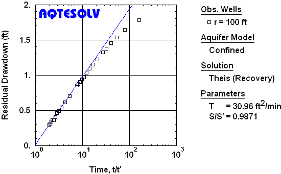
The foregoing figures illustrate the use of the three recovery test methods in the analysis of a field example reported in the Ground Water Manual (USBR 1995). The results show that one may obtain consistent aquifer property estimates with all three techniques.
Learn more about the three methods of recovery analysis in Aquifer Testing 101 at the AQTESOLV web site.
![]() |
| Method 1: Combined analysis of drawdown and recovery data. |
![]() |
| Method 2: Analysis of residual drawdown data. |
![]() |
| Method 3: Analysis using Agarwal (1980) method. |
Learn more about the three methods of recovery analysis in Aquifer Testing 101 at the AQTESOLV web site.
Monday, December 31, 2007
Wellfield Simulations
This will be my last post for 2007, so let me begin by expressing my sincere appreciation and gratitude to all of you who have either become new AQTESOLV customers or continued to support the software by upgrading in the past year. As always I'm working hard to add new features that will maintain AQTESOLV's status as the leading software for aquifer test analysis.
As many of you already know, AQTESOLV includes the capability to model more than one pumping well in either pumping test analyses or predictive simulations. You may enter a variable pumping rate schedule for each well. For example, you can use the multiple pumping well feature to predict total drawdown in a wellfield as shown in the contour plot.
Another use of this multi-well feature would be to include the effect of more than one pumping well in the analysis of a pumping test (e.g., a domestic well that turns on and off during your test). Image wells can be simulated in the same way.
Best wishes for a happy and healthy New Year!
As many of you already know, AQTESOLV includes the capability to model more than one pumping well in either pumping test analyses or predictive simulations. You may enter a variable pumping rate schedule for each well. For example, you can use the multiple pumping well feature to predict total drawdown in a wellfield as shown in the contour plot.
Another use of this multi-well feature would be to include the effect of more than one pumping well in the analysis of a pumping test (e.g., a domestic well that turns on and off during your test). Image wells can be simulated in the same way.
Best wishes for a happy and healthy New Year!
Labels:
features,
multiple pumping wells,
prediction,
tips,
wellfield simulation
Saturday, April 21, 2007
Horizontal Wells in AQTESOLV
One of the new features introduced in AQTESOLV/Pro v4.0 is a solution for a pumping test conducted in an anisotropic confined aquifer with a horizontal well (Daviau et al. 1985). With this solution, you may analyze drawdown data from fully or partially penetrating observation wells to determine the following aquifer properties: T (transmissivity), S (storativity) and Kz/Kr (hydraulic conductivity anisotropy ratio).The horizontal well solution in AQTESOLV has been benchmarked against published well function values (Clonts and Ramey 1986) as shown in the accompanying figure.
AQTESOLV provides options for uniform-flux and infinite-conductivity conditions at the horizontal well as well as variable rates, recovery, multiple horizontal wells and multiple observation wells.
Labels:
features,
horizontal wells,
pumping tests,
tips
Subscribe to:
Posts (Atom)