Interview With C.V. Theis

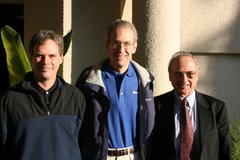
Kick back and enjoy a lively and engaging video interview of Charles Vernon Theis who introduced the concept of transient flow to the interpretation of pumping tests. His seminal paper from 1935, "The relation between the lowering of the piezometric surface and the rate and duration of discharge of a well using groundwater storage," is familiar to all hydrogeologists. Learn more about his many accomplishments as well as the groundwater scientists with whom he worked during his long career at the U.S. Geological Survey.

Get more details on the Theis solution at the AQTESOLV website.

Follow AQTESOLV on LinkedIn and Google+ for more updates on aquifer testing!

Classic USGS Pumping Test Video

Check out this classic video of a pumping test conducted by the U.S. Geological Survey in the Little Plover River basin in Wisconsin, USA.

The USGS study made news in a Milwaukee Sentinel article in 1961. A new study in this river basin is underway.

Follow AQTESOLV on LinkedIn and Google+ for more news on aquifer testing!

Checking Your Cooper and Jacob Match

Groundwater hydrologists use the Cooper and Jacob (1946) solution to determine the aquifer properties of a nonleaky confined aquifer using drawdowns measured during a constant-rate pumping test. The approximate method of Cooper and Jacob derives from the Theis (1935) type-curve method when the variable u in the Theis well function, w(u), is sufficiently small (i.e., time is large or radius is small).

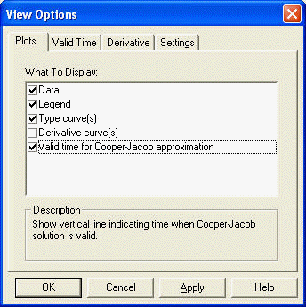
AQTESOLV has built-in tools to check the validity of analyses performed with the Cooper and Jacob method and to assist you with visual curve matching. First, you can superimpose on your plot the time when u is less than a critical value. Choose View>Options>Plots tab and check the option for Valid time for Cooper-Jacob approximation (Figure 1).

Figure 1. Check option to display valid time for Cooper and Jacob solution.

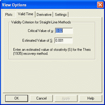
Click the Valid Time tab to set the critical value of u (Figure 2). A critical value between 0.01 and 0.05 is typical.

Figure 2. Set critical value of u used to check validity of Cooper and Jacob approximation.

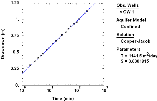
When you activate the valid time option, a dashed vertical line appears on your time-drawdown or composite plot to indicate the time when the Cooper and Jacob approximation meets the critical value of u (Figure 3). The position of the vertical line is a function of T (transmissivity) and S (storage coefficient) as well as radial distance between the pumping and observation wells..

Figure 3. Cooper and Jacob method (blue line) matched to time-drawdown data from constant-rate pumping test (data from Todd 1980). Dashed vertical line indicates time when Cooper and Jacob approximation becomes valid.

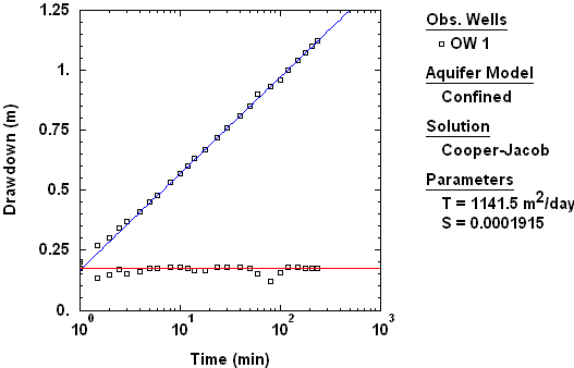
The second way that you may evaluate the proper application of the Cooper and Jacob method using AQTESOLV is through derivative analysis. After superimposing the derivative on your semilog plot of drawdown versus time, match the Cooper and Jacob straight line to drawdowns corresponding to the derivative plateau, i.e., during the period of infinite-acting radial flow (Figure 4).

Figure 4. Cooper and Jacob method (blue line) matched to drawdown data during period of infinite-acting radial flow when derivative reaches plateau (red line).

Use these two techniques to obtain more reliable results when using the Cooper and Jacob method. Get AQTESOLV and start applying these powerful tools in your next pumping test interpretation!

Visit the AQTESOLV Knowledge Base to find more tips on the using the software. The AQTESOLV documentation also includes a number of examples illustrating the use of the Cooper and Jacob straight-line method.

We invite you to follow HydroSOLVE on LinkedIn and Google+!

IARF and the Cooper and Jacob Method

Groundwater hydrologists routinely use the pumping test interpretation method of Cooper and Jacob (1946), a straight-line approximation of the Theis (1935) type-curve solution, to estimate the hydraulic properties of nonleaky confined aquifers from drawdown data measured during the period of infinite-acting radial flow (IARF) when drawdown changes linearly with the logarithm of time. One expects to find IARF after the dissipation of early-time phenomena (e.g., wellbore storage) and prior to the advent of late-time effects such as aquifer boundaries.

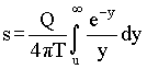
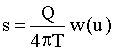
Consider the well-known Theis solution for a constant-rate pumping test in a nonleaky confined aquifer of infinite extent:

..... (1)

..... (2)

..... (3)

..... (4)

where s is drawdown [L], Q is pumping rate [L³/T], T is transmissivity [L²/T], t is time [T], r is radial distance [L] and S is storage coefficient [-].

The Cooper and Jacob method approximates the Theis well function, w(u), by truncating the infinite series in (4) after the first two terms:

..... (5)

The approximation in (5) assumes that u is small, i.e., t is large and r is small. It is precisely when (5) is valid that infinite-acting radial flow is identified from drawdown data.

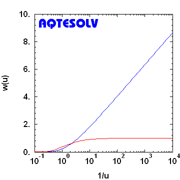
How small should u be for (5) to be valid? The threshold for IARF (i.e., when Cooper and Jacob becomes valid) is often given as u ≤ 0.05 (Driscoll 1986) or u ≤ 0.01 (Kruseman and de Ridder 1994); however, we can see for ourselves when (5) is valid by plotting w(u) versus 1/u (dimensionless drawdown versus dimensionless time) on semilog axes and looking for a constant logarithmic derivative plateau (Figure 1).

Figure 1. Theis (1935) solution (blue curve) plotted as w(u) versus 1/u on semilog axes. Logarithmic derivative shown by red curve.

It is evident from Figure 1 that the slope of the drawdown and the value of the derivative are each essentially constant when 1/u ≥ 50. Hence, when u ≤ 0.02, the Cooper and Jacob approximation of the Theis well function is safe to use. Figure 1 demonstrates just how useful derivative analysis can be for the detection of the IARF regime.

Visit Aquifer Testing 101 to learn more about pumping test interpretation with more examples of infinite-acting radial flow.

Follow HydroSOLVE on LinkedIn and Google+!

Infinite-Acting Radial Flow Regime

At the outset of interpreting a pumping test, an important feature to detect in the response data is infinite-acting radial flow. During infinite-acting radial flow, steady pumping in a nonleaky confined aquifer of infinite extent produces late-time drawdown that changes with the logarithm of time since pumping began. Infinite-acting behavior occurs after wellbore storage effects have dissipated and before the influence of aquifer boundaries. One may observe this flow regime by plotting the familiar Theis (1935) solution on semilog axes (Figure 1); at late time, a graph of dimensionless drawdown, w(u), versus dimensionless time, 1/u, plots as a straight line and the logarithmic derivative is constant.

 

Figure 1. Infinite-acting radial flow in a nonleaky confined aquifer illustrated with Theis (1935) solution (dimensionless drawdown and dimensionless derivative shown by blue and red curves, respectively).

This late-time behavior of the Theis model is well known to groundwater hydrologists. The period of infinite-acting radial flow is the basis for the tried-and-true Cooper and Jacob (1946) method which one may use to find the transmissivity and storage coefficient of a nonleaky confined aquifer by matching a straight line to late-time drawdown data from a constant-rate pumping test plotted on semilog axes.

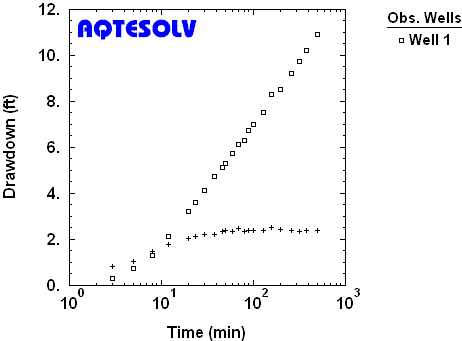
A derivative plot is very useful for detecting the infinite-acting radial flow regime under steady pumping conditions. One starts by looking for a derivative plateau (constant derivative) to tentatively identify infinite-acting radial flow. For example, the response data from a constant-rate pumping test shown in Figure 2 suggest that infinite-acting radial flow conditions are present after approximately 30 minutes of pumping once the derivative stabilizes.

Figure 2. Derivative plot of drawdown (squares) and derivative (crosses) measured in an observation well during constant-rate pumping test in a nonleaky confined aquifer (Walton 1962).

Note that the derivative plateau in Figure 2 exhibits some noise; derivative fluctuation at the plateau is common in the application of derivative analysis, but the presence of a near-constant derivative in this example is clear and corresponds to the emergence of a well-defined straight line in the drawdown data.

The foregoing results suggest that the derivative plot is an indispensable tool for aquifer test interpretation; however, the mere existence of a derivative plateau does not immediately confirm infinite-acting radial flow conditions. For example, an aquifer limited by a no-flow boundary can produce a constant derivative that is not diagnostic of the infinite-acting radial flow regime. In such a situation, geologic mapping of lithologic contacts, faults and other low-permeability features would be invaluable in making a correct interpretation.

Visit Aquifer Testing 101 for a catalog of derivative plot signatures with more examples of infinite-acting radial flow in pumping tests.

Follow HydroSOLVE on LinkedIn!

Curve Matching With Multiple Observation Wells

When you analyze a pumping test with more than one observation well, AQTESOLV matches one set of aquifer properties to the drawdown data from all of the wells in your data set.

One set of aquifer properties matched to two observation wells from a constant-rate pumping test in an unconfined aquifer with delayed yield.

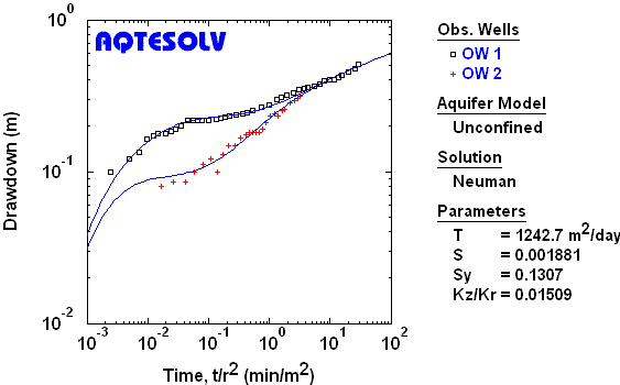
In the figure shown above, the curve-fitting analysis determines the properties of an unconfined aquifer with delayed yield from the two observation wells displayed on the graph.

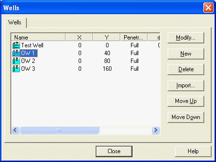
Of course, if your data set has multiple observation wells, you may match wells individually or in groups with AQTESOLV as well. To perform visual curve matching on selected wells, choose Wells from the Edit menu to see all of the wells in your data set. Right click over a well in the list and choose Hide Observations to turn off the display of the well; to turn on the display a previously hidden well, choose Show Observations when you right click over a well.

Choose Edit>Wells to add, modify or delete wells from an AQTESOLV data set.

To select more than one well at a time, hold down the Ctrl key when clicking on wells in the list shown above.

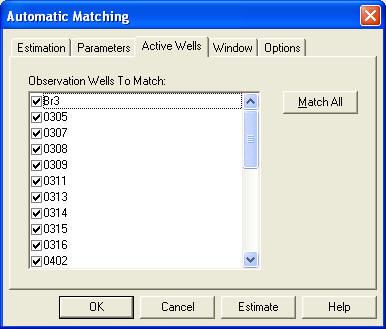
AQTESOLV allows you to select which wells to use for automatic curve matching, too. Choose Automatic from the Match menu and click the Active Wells tab. Remove the check next to any well that you wish to ignore during automatic matching.

Choose Match>Automatic>Active Wells to select wells to match with automatic curve matching.

Selections in the Active Wells list shown above only affect the wells used for automatic matching, not the display of well data.

Visit the Support Center and the Knowledge Base at the AQTESOLV website for additional tips and examples.

Analyzing Pumping Tests With Multiple Observation Wells

AQTESOLV allows you to analyze pumping tests with more than one observation well. For example, Figure 1 shows the interpretation of drawdown data recorded in the pumped well and three observations wells during a constant-rate pumping test conducted in a nonleaky confined channel aquifer (near Estevan, Saskatchewan, Canada).

Figure 1. Constant-rate pumping test in nonleaky confined channel aquifer (Walton 1970).

Prior to late-time boundary effects, one observes infinite-acting aquifer conditions in the drawdown response at all wells (Figure 1).

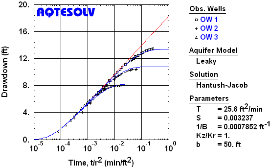
Analysis of multiple observation wells is not limited to nonleaky confined aquifers. In the following figure, we see the analysis of drawdown data from a constant-rate pumping test in a leaky confined aquifer with three observation wells.

Figure 2. Constant-rate pumping test in leaky confined aquifer (USBR 1995).

Interpretation of this test uses the Hantush and Jacob (1955) method for a leaky confined aquifer with incompressible aquitard(s). Prior to the onset of leakage, the aquifer behaves like a nonleaky confined aquifer of infinite extent as shown in Figure 2 by the superimposed Theis (1935) solution (red curve).

We can use AQTESOLV to analyze multi-well tests in phreatic aquifers, too. For example, two  fully penetrating observation wells are used for the interpretation of a constant-rate pumping test in an unconfined aquifer with delayed yield near Gironde, France (Figure 3).

Figure 3. Constant-rate pumping test in unconfined aquifer with delayed yield (Neuman 1975).

Analysis in the example above is performed with the Neuman (1974) method for an anisotropic water-table aquifer with delayed gravity response; one can see from the composite plot how the shape of the drawdown response is affected by radial distance from the pumping well (Figure 3).

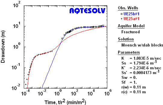
Figure 4 shows the interpretation of a multi-well constant-rate pumping test in a double-porosity fractured aquifer using a solution by Moench (1984).

Figure 4. Constant-rate pumping test in double-porosity fractured aquifer (Moench 1984).

In the example above, the blue curve on the composite plot shows the fit to drawdown data from the pumped well while the red curve is matched to observation well data.

In each of the preceding examples, one set of aquifer properties was used to match drawdown data from all observation wells in a data set. At times, however, you may wish to match only a few wells by themselves. You may accomplish this task using either visual or automatic curve matching in AQTESOLV.

Sometimes you start out with only one or two observation wells in a data set and wish to add more wells later. Adding observation wells is easy with AQTESOLV. Choose Wells from the Edit menu and click New to enter data for a new well.

To find worked examples of pumping tests with multiple observation wells, check out the AQTESOLV Help file/manual or visit the Application Gallery at the AQTESOLV web site.

Entering Pumping Rates Into AQTESOLV

Entering pumping rates from an aquifer test into AQTESOLV requires little effort. The first thing to remember is that all pumping rates are entered as a sequence of constant-rate steps. For each step, enter the time when the step begins (as elapsed time since the start of the test) with the corresponding pumping rate. For your convenience, AQTESOLV provides options to type the rates into a spreadsheet, import them from a file or copy/paste them from another spreadsheet.

Constant-Rate Test

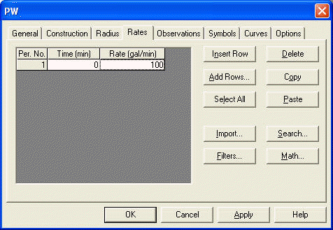
For a constant-rate pumping test, you only need to enter one rate into AQTESOLV. For example, if the pumping rate during a constant-rate test is 100 gpm (gallons-per-minute), enter the rate as shown below.

Pumping rate entry for a constant-rate test.

Note that there's no need to duplicate the rate in the spreadsheet after the first entry. AQTESOLV assumes that the rate doesn't change until you add a new one. Duplicating rates in successive rows of the spreadsheet only serves to slow down calculations.

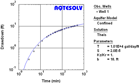
The following figure shows an interpretation of drawdown data from a constant-rate pumping test with the Theis (1935) type-curve method.

Analysis of drawdown data from constant-rate pumping test.

Constant-Rate Test With Recovery

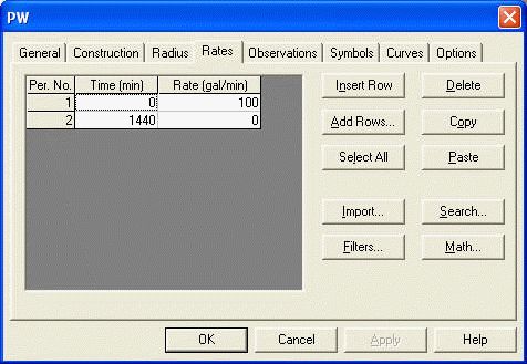
Now consider a constant-rate pumping test with recovery. For this case, enter the constant-rate portion of the test as above and add a row to the rates spreadsheet to indicate the start of recovery. For example, if pumping at 100 gpm ceases after 24 hours (1440 minutes), enter the constant rate and recovery periods as follows.

Pumping rate entry for a constant-rate test with recovery.

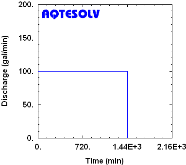
The next graph shows the rate history for the example above. The rate during the pumping test is a constant 100 gpm. After one day (1440 minutes), the test ends and the rate is zero during recovery.

Rate history for constant-rate test with recovery.

As before, do not duplicate pumping rates in successive rows of the rates spreadsheet. Between 0 and 1440 minutes, AQTESOLV recognizes that the constant rate is 100 gpm. AQTESOLV knows from the data entered that the rate after 1440 minutes is zero during recovery.

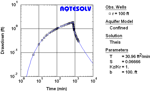
The plot below illustrates the analysis of drawdown and recovery data from a constant-rate pumping test with recovery.

Analysis of constant-rate pumping test with recovery.

Variable-Rate Test

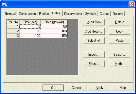
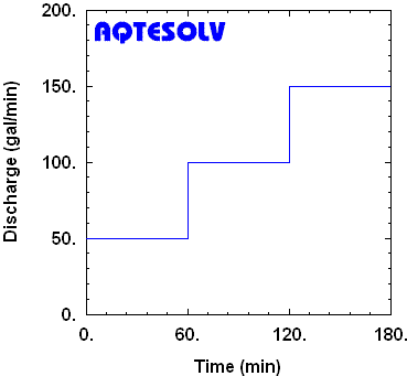
Entering pumping rates for a variable-rate test is likewise straightforward. Enter a new rate into AQTESOLV when the rate changes. For example, consider a step-drawdown test consisting of three one-hour steps of 50, 100 and 150 gpm. As before, the first step starts at an elapsed time of zero. The second and third steps begin at 60 and 120 minutes, respectively.

Pumping rate entry for step-drawdown test.

The rate history for this step-drawdown test example is illustrated in the graph below.

Rate history for step-drawdown test.

Enter only one row per step in the rates spreadsheet to indicate when the step begins. During each step, the pumping rate is assumed to remain constant.

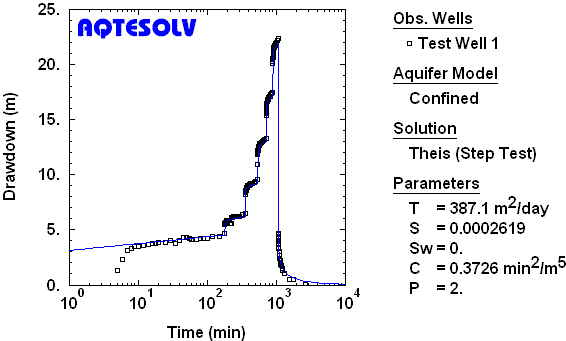
Interpretation of a step-drawdown test with recovery is shown in the following figure.

Interpretation of drawdown and recovery data from a step-drawdown test.

Visit the Knowledge Base at the AQTESOLV website for more helpful tips on using the software!

Distance-Drawdown Analysis

Distance-drawdown analysis is a useful technique for estimating aquifer properties when drawdown measurements are taken during a pumping test at several observation wells located at different radial distances from the control (pumped) well. To perform distance-drawdown analysis, one plots a single drawdown observation per well, each recorded at the same time since the start of pumping, on a graph of drawdown versus radial distance.

Most of us are familiar with estimating an aquifer's transmissivity and storativity from distance-drawdown data using the Cooper and Jacob (1946) method as shown in the following figure.

Distance-drawdown analysis for an unconfined aquifer.

Did you know that you may perform distance-drawdown analysis with pumping test methods in AQTESOLV other than Cooper and Jacob? For example, you may match distance-drawdown data with the Hantush and Jacob (1955) method for a leaky confined aquifer (see figure below).

Distance-drawdown plot for a leaky confined aquifer.

To display a distance-drawdown graph in AQTESOLV, choose Distance-Drawdown from the View menu. The Distance-Drawdown option is active when you have more than one observation well in your data set. If your data set includes more than one pumping well, the Distance-Drawdown option is inactive as distance-drawdown analysis assumes radially symmetric flow around a single pumping well; however, you may use AQTESOLV to prepare contour plots of drawdown (plan and cross section) when multiple pumping wells are present.

To learn more about AQTESOLV, take the guided tour or download the demo!

Plot Orientation in AQTESOLV

Many groundwater hydrologists prefer plotting drawdown data from a pumping test with the origin placed in the upper left corner of the graph. When formatted this way, a graph shows drawdown increasing downward.

Analysis of drawdown and recovery from a pumping test in a confined aquifer.

To have AQTESOLV orient your drawdown plot in this manner, choose Format from the View menu and check Origin in Upper Left.

For additional AQTESOLV tips, visit the Knowledge Base and Examples at the AQTESOLV Support Center.

Catalog of Derivative Plots

Derivative analysis is a powerful diagnostic technique for the interpretation of data from pumping tests. Use of the derivative in pumping test analysis can highlight many flow regime features that otherwise may be hard to discover when inspecting drawdown data alone.

A catalog of derivative plots, showing the theoretical drawdown and derivative signatures on log-log axes for different flow regimes, is a useful reference to the practicing hydrogeologist when performing derivative analysis. For example, Figure 1 shows the drawdown and derivative response for a finite-diameter pumping well with wellbore storage in an infinite nonleaky confined aquifer.

Figure 1. Wellbore storage flow regime, infinite nonleaky confined aquifer.

One observes the wellbore storage flow regime at early time when the drawdown and derivative curves both exhibit unit (1:1) slopes (Figure 1). Radial flow in an infinite-acting aquifer shows up as a plateau on the derivative response.

An extensive catalog of derivative plots is available at the Aquifer Testing 101 section of the AQTESOLV web site to help you with derivative analysis. Use the catalog to become familiar with the derivative plot signatures for various well/aquifer geometries corresponding to different flow regimes.

Importance of Smoothing Derivative Data

Derivative analysis is a powerful diagnostic tool that enhances the interpretation of pumping test data. Hydrogeologists use the technique to identify flow regimes, discern boundary conditions and refine the selection of aquifer models.

Derivatives are not measured directly in the field; rather, they are computed by numerical differentiation from drawdowns collected during a pumping test. Straightforward calculation of the derivative from neighboring drawdown measurements typically leads to noisy derivative data. Therefore, smoothing routines are employed to obtain a cleaner derivative signal (Bourdet et al. 1989; Spane and Wurstner 1993).

To appreciate the importance of derivative smoothing, consider field data measured in a deep piezometer during a constant-rate pumping test performed in an unconfined aquifer (Kruseman and de Ridder 1994). Figure 1 is a derivative plot for the piezometer showing drawdown (squares) and derivatives (crosses) computed without smoothing (nearest neighbor method). Without smoothing, the derivative data provide little useful information for the interpretation of this test.

Figure 1. Derivative plot showing derivatives computed without smoothing.

Application of the Bourdet method to smooth the derivatives leads to a derivative plot with useful information (Figure 2). The trough in the derivative curve shown in Figure 2 is typical for an unconfined aquifer with delayed yield. The derivative signature suggests the possibility of using a mathematical model by Neuman (1974) to interpret the data.

Figure 2. Derivative plot showing derivatives computed with Bourdet smoothing.

AQTESOLV features three smoothing methods for computing derivatives including the Bourdet and Spane methods.

More information on derivative analysis is available at Aquifer Testing 101.

Hydraulics of Wells

Hydraulics of Wells by M. S. Hantush (1964) is available for download. This classic work is a recommended reference for the bookshelf of every practicing hydrogeologist.

To find more aquifer testing materials including other links to downloadable resources, check out my reference list at the Aquifer Testing 101 web site.

Horizontal Wells in AQTESOLV

One of the new features introduced in AQTESOLV/Pro v4.0 is a solution for a pumping test conducted in an anisotropic confined aquifer with a horizontal well (Daviau et al. 1985). With this solution, you may analyze drawdown data from fully or partially penetrating observation wells to determine the following aquifer properties: T (transmissivity), S (storativity) and Kz/Kr (hydraulic conductivity anisotropy ratio).

The horizontal well solution in AQTESOLV has been benchmarked against published well function values (Clonts and Ramey 1986) as shown in the accompanying figure.

AQTESOLV provides options for uniform-flux and infinite-conductivity conditions at the horizontal well as well as variable rates, recovery, multiple horizontal wells and multiple observation wells.