 |
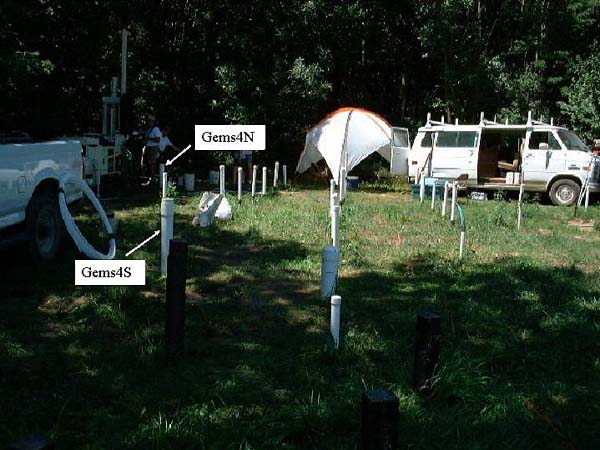
| GEMS Research Site (Butler et al. 2000) |
Wednesday, July 20, 2011
Summit in Lawrence, Kansas
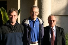
On today's date in 1969, Neil Armstrong made history by becoming the first man to walk on the moon. Forty-two years later, July 20th marks another red-letter day with the conclusion of the 1st Lawrence Summit hosted by Jim Butler and attended by Dan Kelleher and myself. The summit met its primary goal of laying the groundwork for future aquifer testing short courses around the world.
Unforgettable moments during the visit included a tour of the venerable Kansas Geological Survey and its GEMS research site, a view of the Allen Field House from Jim's bleacher seats ("Rock, Chalk, Jayhawk!") and a reverential pilgrimage to the James Naismith ("Inventor of Basketball") Memorial. Without question, though, the unsurpassed highlight of the summit was the delightful sushi dinner served to perfection by Jim's daughter, Mai. Many thanks to Jim and wife Yun for their warm hospitality throughout the Lawrence Summit!


Thursday, July 14, 2011
Agarwal Recovery Method
In yesterday's post, I presented three different methods for analyzing recovery tests. Today, I will focus on the Agarwal recovery method which has been used by petroleum engineers for over 30 years. Agarwal (1980) devised a simple yet powerful data transformation for the interpretation of recovery tests. The transformation, known as Agarwal equivalent time, allows one to analyze recovery data with standard type curves developed for drawdown data.
The following figure illustrates the simplicity of the Agarwal method in the analysis of a recovery test. In this example, I matched the familiar Theis type curve, normally applied to drawdown data, to estimate aquifer properties from recovery test data (USBR 1995).
Many different pumping test solutions may be used in conjunction with the Agarwal technique as well as diagnostic methods such as derivative analysis. The figure below shows recovery and derivative data matched together with the Cooper-Jacob straight-line solution.
Recovery test analysis with the Agarwal equivalent-time method is available in AQTESOLV v4.x. This advanced aquifer test analysis software allows you to estimate aquifer properties by matching both recovery and derivative data together.
Learn more about the Agarwal method in Aquifer Testing 101 at the AQTESOLV web site.
The following figure illustrates the simplicity of the Agarwal method in the analysis of a recovery test. In this example, I matched the familiar Theis type curve, normally applied to drawdown data, to estimate aquifer properties from recovery test data (USBR 1995).
 |
| Agarwal recovery analysis using Theis (1935) solution. |
 |
| Agarwal recovery analysis using Cooper-Jacob (1946) solution with derivative. |
Learn more about the Agarwal method in Aquifer Testing 101 at the AQTESOLV web site.
Wednesday, July 13, 2011
Analyzing Recovery Tests
Did you know that AQTESOLV v4.x provides three different methods for the analysis of recovery tests?
The foregoing figures illustrate the use of the three recovery test methods in the analysis of a field example reported in the Ground Water Manual (USBR 1995). The results show that one may obtain consistent aquifer property estimates with all three techniques.
Learn more about the three methods of recovery analysis in Aquifer Testing 101 at the AQTESOLV web site.
 |
| Method 1: Combined analysis of drawdown and recovery data. |
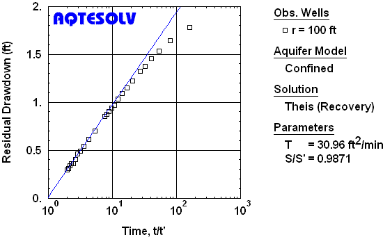 |
| Method 2: Analysis of residual drawdown data. |
|
| Method 3: Analysis using Agarwal (1980) method. |
Learn more about the three methods of recovery analysis in Aquifer Testing 101 at the AQTESOLV web site.
Sunday, November 1, 2009
Groundwater Mounding
Upon its release in 2006, AQTESOLV/Pro v4.0 became the first aquifer testing software to feature groundwater mounding calculators that predict the transient rise and decay of the water table beneath rectangular and circular recharge areas (Hantush 1967). Using AQTESOLV, you may compute the maximum rise of the water table and generate contours of a groundwater mound with ease.
 The example plot (above) shows a 3-D contour plot of a groundwater mound developed around a hypothetical rectangular recharge area. Applications for the groundwater mounding calculators in AQTESOLV include infiltration from septic systems and recharge from stormwater impoundments.
Visit the AQTESOLV web site for more information on the Hantush (1967) solutions for groundwater mounding prediction.

Visit the AQTESOLV web site for more information on the Hantush (1967) solutions for groundwater mounding prediction.
Saturday, June 20, 2009
ASTM "Standards"
ASTM publishes "standards" on many subjects including aquifer test analysis. ASTM D5912-96 (2004) entitled Standard Test Method for (Analytical Procedure) Determining Hydraulic Conductivity of an Unconfined Aquifer by Overdamped Well Response to Instantaneous Change in Head (Slug) is one such ASTM standard. You'll spend $32 to obtain a copy of this four-page standard from ASTM, but don't expect to get completely accurate information for your investment.
ASTM D5912-96 (2004) describes a widely used method of slug test analysis devised by Bouwer and Rice (1976). The standard contains an equation (ASTM D5912-96 (2004), p. 2, Equation [2]) used in the Bouwer and Rice method to calculate the parameter ln(Re/rw) when D (the aquifer thickness) is greater than H (the penetration of the well) as follows:

The ln(Re/rw) parameter is used in the Bouwer and Rice method to calculate the hydraulic conductivity K from a slug test.
Unfortunately, the above equation from ASTM D5912-96 (2004) is incorrect. The correct form of this equation (Bouwer and Rice 1976, p. 425, Equation [8]) is written as follows:

As one can see from a comparison the two foregoing equations, the ASTM version misplaces the term L/rw and leads to a completely erroneous estimate of ln(Re/rw).
Am I just nitpicking here? I don't think so. It's hardly unreasonable to expect thorough attention to detail from a publication put forth as a "standard" such as ASTM D5912-96 (2004). Certainly, the basic equations that are central to such a standard should be checked carefully and published without error. ASTM standards purportedly go through a rigorous review process. Yet ASTM D5912-96 (2004), adopted in 1996 and subsequently reapproved in 2004, still contains the flawed equation. One is left to wonder how many other "standards" relied upon for aquifer testing contain similar fundamental errors.
ASTM D5912-96 (2004) describes a widely used method of slug test analysis devised by Bouwer and Rice (1976). The standard contains an equation (ASTM D5912-96 (2004), p. 2, Equation [2]) used in the Bouwer and Rice method to calculate the parameter ln(Re/rw) when D (the aquifer thickness) is greater than H (the penetration of the well) as follows:

The ln(Re/rw) parameter is used in the Bouwer and Rice method to calculate the hydraulic conductivity K from a slug test.
Unfortunately, the above equation from ASTM D5912-96 (2004) is incorrect. The correct form of this equation (Bouwer and Rice 1976, p. 425, Equation [8]) is written as follows:

As one can see from a comparison the two foregoing equations, the ASTM version misplaces the term L/rw and leads to a completely erroneous estimate of ln(Re/rw).
Am I just nitpicking here? I don't think so. It's hardly unreasonable to expect thorough attention to detail from a publication put forth as a "standard" such as ASTM D5912-96 (2004). Certainly, the basic equations that are central to such a standard should be checked carefully and published without error. ASTM standards purportedly go through a rigorous review process. Yet ASTM D5912-96 (2004), adopted in 1996 and subsequently reapproved in 2004, still contains the flawed equation. One is left to wonder how many other "standards" relied upon for aquifer testing contain similar fundamental errors.
Tuesday, April 28, 2009
AQTESOLV in Boston
Today marks the beginning of our three-day Advanced Aquifer Testing Techniques Featuring AQTESOLV: New Concepts, Field Methods and Data Analysis Procedures short course at the Waltham Wood Conference Center outside of Boston, MA. Presented in cooperation with the Midwest Geosciences Group, we have been offering this course every year since 2006. The course covers aquifer testing topics pertaining to slug tests and pumping tests. As part of each day's activities, course participants gain hands-on experience with the AQTESOLV software using data from real-life field investigations conducted in a variety of hydrogeologic settings.
 Last year (2008) seemed to come and go very quickly owing to an extremely busy schedule! We presented our three-day aquifer testing course featuring AQTESOLV in San Antonio, TX to a large audience and also taught well-attended two-day seminars in Waterloo, ON, Canada as well as Ft. Collins, CO. A wonderfully exciting time for me was a three-week period in November and December 2008 when I traveled to Australia to participate in the instruction of short courses on fractured bedrock in Melbourne and Sydney.
 Last year (2008) seemed to come and go very quickly owing to an extremely busy schedule! We presented our three-day aquifer testing course featuring AQTESOLV in San Antonio, TX to a large audience and also taught well-attended two-day seminars in Waterloo, ON, Canada as well as Ft. Collins, CO. A wonderfully exciting time for me was a three-week period in November and December 2008 when I traveled to Australia to participate in the instruction of short courses on fractured bedrock in Melbourne and Sydney.
Monday, December 31, 2007
Wellfield Simulations
This will be my last post for 2007, so let me begin by expressing my sincere appreciation and gratitude to all of you who have either become new AQTESOLV customers or continued to support the software by upgrading in the past year. As always I'm working hard to add new features that will maintain AQTESOLV's status as the leading software for aquifer test analysis.
 As many of you already know, AQTESOLV includes the capability to model more than one pumping well in either pumping test analyses or predictive simulations. You may enter a variable pumping rate schedule for each well. For example, you can use the multiple pumping well feature to predict total drawdown in a wellfield as shown in the contour plot.
Another use of this multi-well feature would be to include the effect of more than one pumping well in the analysis of a pumping test (e.g., a domestic well that turns on and off during your test). Image wells can be simulated in the same way.
Best wishes for a happy and healthy New Year!

Another use of this multi-well feature would be to include the effect of more than one pumping well in the analysis of a pumping test (e.g., a domestic well that turns on and off during your test). Image wells can be simulated in the same way.
Best wishes for a happy and healthy New Year!
Subscribe to:
Posts (Atom)